Genome Annotation with Prokka
Overview
After taxonomy and MLST, the next step is to annotate the assembled genome.
Genome annotation is the process of identifying genes and other genomic features in an assembly. These features may include protein-coding genes, rRNA genes, tRNA genes, and other functional elements.
In this lesson, we will use Prokka to annotate the filtered assembly file.
Learning objectives
By the end of this lesson, you should be able to:
- explain what genome annotation means
- activate the
annotationenvironment - run
Prokkaon a filtered assembly file - identify important Prokka output files
- understand why
.gfffiles are needed for pangenome analysis - download annotation files from the server
Input file
In the previous lessons, we created a filtered assembly file:
assemblies/S1_contigs_filtered.fastaCheck that the file exists:
ls assembliesYou should see:
S1_contigs_filtered.fastaFor this lesson, we will use the filtered assembly file:
assemblies/S1_contigs_filtered.fastaActivate the annotation environment
Activate the annotation environment:
conda activate annotationCheck that Prokka is available:
prokka --versionRun Prokka
Run Prokka on the filtered assembly:
prokka \
  --outdir annotation \
  --force \
  --cpus 4 \
  --prefix S1 \
  --locustag S1 \
  assemblies/S1_contigs_filtered.fasta
Understanding the Prokka command
| Option | Meaning |
|---|---|
prokka |
Runs the Prokka annotation tool |
--outdir annotation |
Output directory |
--force |
Overwrite the output directory if it already exists |
--cpus 4 |
Use 4 CPU threads |
--prefix S1 |
Prefix for output file names |
--locustag S1 |
Prefix for gene locus tags |
assemblies/S1_contigs_filtered.fasta |
Input filtered assembly file |
Once command started running you will see below message: 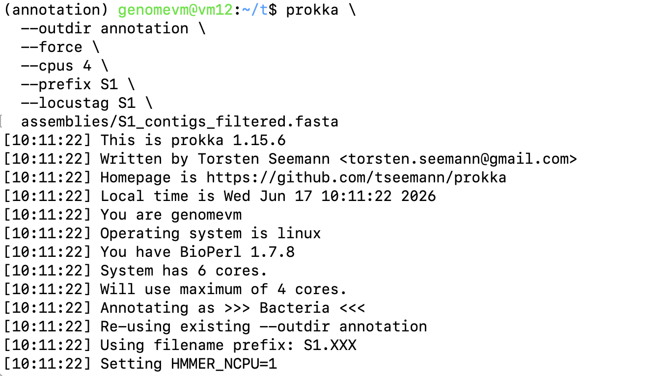
The option --force allows Prokka to overwrite the existing annotation folder.
Use it carefully if you already have files in the annotation directory.
Once you are done working here deactivate the environment:
conda deactivateCheck Prokka outputs
List the annotation directory:
ls annotationYou should see files such as:
S1.err
S1.faa
S1.ffn
S1.fna
S1.fsa
S1.gbk
S1.gff
S1.log
S1.sqn
S1.tbl
S1.tsv
S1.txt
Important Prokka output files
| File | Description |
|---|---|
S1.gff |
Main annotation file; used later for pangenome analysis |
S1.gbk |
GenBank format annotation |
S1.faa |
Protein sequences |
S1.ffn |
Nucleotide sequences of predicted coding genes |
S1.fna |
Contig sequences |
S1.tsv |
Tab-separated annotation table |
S1.txt |
Annotation summary |
S1.log |
Prokka log file |
Example Prokka summary
After running:
cat annotation/S1.txtyou may see output like this:
organism: Genus species strain
contigs: 80
bases: 3912637
CDS: 3449
rRNA: 5
tRNA: 28
tmRNA: 1
Interpreting this summary
| Field | Value | Meaning |
|---|---|---|
organism |
Genus species strain |
Organism name used by Prokka |
contigs |
80 |
Number of contigs in the assembly |
bases |
3,912,637 |
Total assembly size in base pairs |
CDS |
3,449 |
Number of predicted coding sequences |
rRNA |
5 |
Number of ribosomal RNA genes |
tRNA |
28 |
Number of transfer RNA genes |
tmRNA |
1 |
Number of transfer-messenger RNA genes |
This means Prokka predicted 3,449 coding sequences from an assembly containing 80 contigs and approximately 3.91 Mbp of sequence.
How many coding sequences were predicted in sample S1?
The number of predicted coding sequences is:
3449What is the total assembly size reported by Prokka?
The total assembly size is:
3912637 bpThis is approximately:
3.91 MbpDownload annotation files from the server
If you are working on a remote server, download the annotation folder to your local computer.
From your local desktop terminal, run:
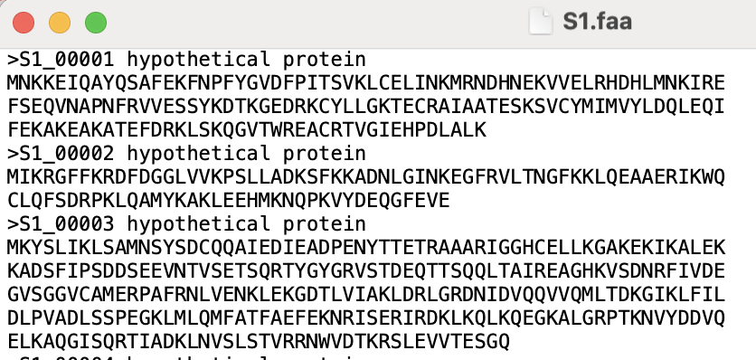
scp -r genomevm@172.28.28.12:~/tanzim/annotation .scp -r genomevm@172.28.28.12:~/tanzim/`annotation` .This downloads the full annotation directory to your current local folder. Now open the desired file S1.ffn or S1.faa or S1.gff
Open S1.ffn using Notepad++, VS Code, or another text editor.
Use:
open S1.ffnUse:
xdg-open S1.ffn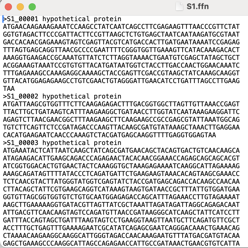
Open the Prokka summary file.
How many coding sequences were predicted?
The answer depends on your dataset. Check the coding sequence count in:
annotation/S1.txtWhy is the GFF file important?
The .gff file combines genome sequence information with gene annotation information.
In this course, the .gff file will be used later for pangenome analysis.
S1.gff → pangenome analysisWhich Prokka output file will be used for pangenome analysis?
The file used for pangenome analysis is:
annotation/S1.gffCompare annotation with previous results
At this stage, you have several outputs for sample S1.
| Analysis | Output file | Purpose |
|---|---|---|
| Taxonomy | classify/S1.kraken2.report |
Taxonomic identity |
| MLST | classify/S1_mlst.txt |
Sequence type |
| Annotation | annotation/S1.gff |
Gene annotation |
| Annotation summary | annotation/S1.txt |
Summary of predicted features |
Do the taxonomy, MLST, and annotation results look consistent for sample S1?
The results should be interpreted together. Kraken2 gives the likely organism, MLST gives the sequence type if the species has a supported scheme, and Prokka provides predicted genes and functional annotation.
Final directory structure
At the end of this lesson, your directory should look like this:
.
├── assemblies
│   ├── S1_contigs.fasta
│   └── S1_contigs_filtered.fasta
├── classify
│   ├── S1.kraken2.output
│   ├── S1.kraken2.report
│   ├── S1.krona
│   ├── S1.krona.html
│   └── S1_mlst.txt
└── annotation
    ├── S1.faa
    ├── S1.ffn
    ├── S1.fna
    ├── S1.gbk
    ├── S1.gff
    ├── S1.tsv
    └── S1.txt
Practical exercise
Complete the following tasks:
- Activate the
annotationenvironment. - Run
ProkkaonS1_contigs_filtered.fasta. - Check the files inside the
annotationdirectory. - Open
annotation/S1.txt. - Record the number of predicted coding sequences.
- Open
annotation/S1.gff. - Identify why the
.gfffile is important for the next analysis.
Create a small table in your notes:
| Sample | Number of contigs | Number of CDS | rRNA genes | tRNA genes | GFF file |
|---|---|---|---|---|---|
| S1 | annotation/S1.gff |
Fill in the values using:
annotation/S1.txtKey points
- Genome annotation identifies genes and other genomic features.
Prokkais commonly used for bacterial genome annotation.- The main output file for downstream pangenome analysis is
annotation/S1.gff. - The
S1.txtfile contains a useful annotation summary. - Annotation results should be interpreted together with taxonomy and MLST results.
Next step
In the next lesson, we will copy prepared files for multiple samples and use them for AMR, virulence factor, pangenome, and phylogenetic analysis.